[논문 리뷰] Effective Approaches to Attention-based Neural Machine Translation - Luong Attention

이번에는 Luong Attention을 다루고 있는 Effective Approaches to Attention-based Neural Machine Translation이라는 논문에 대해 리뷰해보려고 한다.

원문 링크는 아래와 같다.

Effective Approaches to Attention-based Neural Machine Translation

 

이 논문에서는 일전에 발표되었던 Bahdanau Attention을 다룬 Neural Machine Translation by Jointly Learning to Align and Translate 논문에서 한 단계 더 나아가 다양한 attention 기법들을 제안하고, 직접 결과들을 비교했다.

Bahdanau Attention을 다룬 Neural Machine Translation by Jointly Learning to Align and Translate 논문에 대한 게시글은 하단 링크에서 확인할 수 있다.

[논문 리뷰] Neural Machine Translation by Jointly Learning to Align and Translate - Bahdanau Attention

 

논문에서 제안된 기법들을 간단히 정리해보자면,

 

• Global attention -> Bahdanau Attention과 비슷하지만 더 간단하고, 다양한 방법론 제시
• Local attention
• Input feeding 

으로 나눠질 수 있겠다. 

하나씩 차근차근 살펴보도록 하자.

 

 

Attention-based Models

우선, 앞서 살짝 언급한대로 논문에서는 하단의 두 가지 Attention-based Model을 제안한다.

 

• Global attention : attention이 모든 position에 있는 model
• Local attention : attention이 일부 position에만 있는 model

두 Attention-based Model은 LSTM layer의 top layer의 hidden state $h_t$를 input으로 하며, 이를 통해 context vector $c_t$를 이끌어내는것은 같다.

다만, 어떻게 context vector $c_t$를 이끌어내는지가 다를 뿐이다. 

 

논문에서는 context vector $c_t$가 만들어진 이후의 과정도 설명하는데, 수식은 다음과 같다

Global attention 혹은 Local attention으로 만들어진 context vector $c_t$는 Decoder의 hidden state $h_t$와 concat한 뒤, concat layer에 통과시켜 $\tilde{h_t}$를 만들어내고, 이를 $W_s$에 통과시킨 다음 softmax를 취하여 timestep $t$에서의 단어의 확률을 산출해낸다.

 

 

Global Attention

먼저, Global Attention의 전반적인 그림을 보면서 설명하고자 한다.

Global Attention은 Bahdanau Attention과 비슷하다. 그러나 논문에서는 다양한 score함수를 제안하였다. 

contents-based function과 location-based function을 제안하는데, contents-based function은 다음과 같다.

참고로, concat 함수는 Bahdanau Attention에서 사용했던 함수이다.

이러한 score function을 통해 나온 score는

다음과 같은 과정을 거쳐 alignment vector $a_t$가 된다.

이어서, location-based function은 다음과 같다

 

이렇게 location-based function과 location-based function를 통해 alignment vector $a_t$를 통해 context vector를 구하고, 위에서 언급한 context vector c_t가 만들어진 이후의 과정을 따르면 된다.

 

이후, 논문에서는 Bahdanau Attention과 본인들이 제안하는 Global attention이 다른 점 3가지를 제시한다.

 

1. Bahdanau Attention과 다르게, Encoder와 Decoder에서 모두 LSTM layer의 top layer의 hidden state만 사용
2. Attention Mechanism의 computation path가 간단해짐 
3. concat score function뿐만 아니라, 다양한 score function을 실험해봄

 

 

Local Attention

논문에서는 target word마다 모든 source를 참고하는 Global Attention의 특징은 길이가 긴 문장에서 expensive하고 impractical해질 수 있다는 문제를 제기 한다.

이러한 문제를 해결하기 위해 다음과 같은 Local Attention을 제안한다.

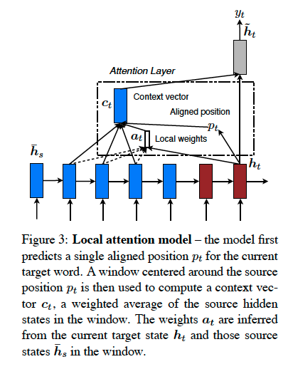
Local Attention을 간략하게 말하자면, target word마다 모든 source를 참고하지 않고, source의 small subset에 집중하여 참고하는 원리이다.

기존 연구들 중에서, soft attention과 hard attention이라는 기법이 제안된 적이 있는데,  soft attention은 expensive conputation이 발생한다는 문제가 있었고, hard attention은 non-differentiable하고 variance-reduction과 강화학습을 필요로 하여 훈련할 때 복잡하다는 단점이 있었다.

저자들은 이러한 문제를 해결하여, soft attention의 expensive conputation을 피하고, hard attention보다 쉽게 학습 가능한 differentiable attention인 Local Attention을 제안한다고 밝힌다.

자세히 알아보면, 전체 source로부터 context vector를 구하지 않고, window $[p_t-D, p_t + D]$에서만 구하는 것이다($D$는

empirically하게 구한다고 한다)

 

 

이러한 Local Attention의 방법으로, 논문에서는 두 개의 방법을 제시한다. 바로

 

• Monotomic alignment (local-m)
• Predictive alignment (local-p)

이다. 

 

Monotomic alignment (local-m)부터 살펴보도록 하겠다.

Monotomic alignment (local-m)는 Global Attention과 거의 비슷하다. $P_t = t$로 하여, Global Attention과 동일한 mechanism이라고 볼 수 있다. alignment vector $a_t$를 구하는 과정도 global과 동일하다.

 

 

이제, Predictive alignment (local-p)를  살펴보겠다.

Predictive alignment (local-p)는 $p_t$를 구하는 방법이 따로 정해져있다. 그 방법은 다음과 같다.

이 과정을 거치게 되면, $p_t$는 0과 $S$사이의 특정 값을 지니게 되고, 이것이 local attention window의 기준점이 되는 것이다.

이후, alignment vector $a_t$를 구해야 하는데, Predictive alignment (local-p)는 이 과정도 따로 정의되어있다. 

우선, $\text{align}(h_t, \bar{h_s})$부분은 기존에 제시된 align function을 그대로 사용하고 $\sigma$의 경우 $\frac{D}{2}$로 설정한다.(논문에서는 이 부분 또한 D를 정한 방법과 동일하게 empirically set이라고 표현하였다.) 이는 p_t를 기준으로 하여 주변 timestep들이 gaussian하게 의미를 가질 것이라고 생각하여 이를 alignment weight에 고려한 것이다.

 

 

Input -feeding Approach

논문에서는 Input-feeding 또한 제시하였는데, 큰 흐름은 다음과 같다.

attention을 이용하여 나온 context vector와 Decoder의 hidden state가 concat되어 나온 $\tilde{h_t}$를, 다음 timestep의 input과 concat하는 것이다.

저자들은 이러한 Input-feeding의 목적으로 두 가지를 제시했는데,

 

• 이전 timestep의 alignment 정보를 알게끔 한다.
• 수평적, 수직적인 deep network를 만들게 한다.

이다. 이 중, 이전 timestep의 alignment 정보를 알게끔 하는것에 대한 부연 설명을 하자면,  원래라면, $\tilde{h_t}$가 softmax에 들어가 그림에서의 $X$가 되는데, 이 softmax 과정에서 손실되는 정보가 발생하게 된다. 따라서, Input feeding을 통해 softmax에서 손실되는 정보를 최소화할 수 있는 것이다.

 

 

Analysis

 

input sequence 길이에 대한 성능 변화이다. BLEU score가 적용되었고, 이를 통해 Attention-based Model이 길이가 긴 sequence에서 좋은 성능을 내는 것을 확인할 수 있다.

논문에서 제안된 방법론들의 조합에 대한 결과이다.

Local Attention, Predictive alignment (local-p), general score 조합이 가장 좋은 성능을 냄을 확인할 수 있다.

Global Attention의 경우, dot score과 조합되는 것이 가장 좋은 성능을 냈음을 확인할 수 있다.

 

실제 alignment와 Attention을 통해 학습된  alignment를 비교하는 AER score 결과이다.

이 결과에서는 local attention이 global attention보다 좋은 결과가 나옴을 확인할 수 있다.

 

---

지금까지  Luong Attention을 다룬 Effective Approaches to Attention-based Neural Machine Translation을 리뷰해보았다.

사실 처음 Attention을 공부할 때 Attention에 다양한 종류가 있는지 몰랐어서, 이를 알게 된 이후 Bahdanau Attention부터 Luong Attention까지 쭉 학습하게 되었다. 

Transformer 구조의 경우 이러한 Attention(Scaled Dot-product attention)으로만 구성되어있기에, 여러번 복습하면서 살펴봐야겠다.